根据信号强度区分细胞核

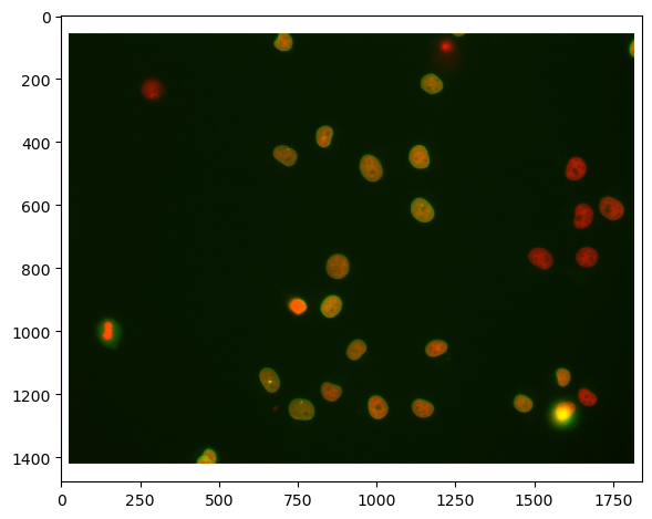
一个常见的生物图像分析任务是根据细胞的信号表达来区分细胞。在这个例子中，我们使用一张表达Cy3和eGFP的细胞核的双通道图像。从视觉上，我们可以很容易地看出一些表达Cy3的细胞核也表达eGFP，而其他的则没有。这个笔记本演示了如何区分在一个通道中分割的细胞核，根据它们在另一个通道中的强度。

import pyclesperanto_prototype as cle
import numpy as np
from skimage.io import imread, imshow
import matplotlib.pyplot as plt
import pandas as pd

cle.get_device()

<Intel(R) Iris(R) Xe Graphics on Platform: Intel(R) OpenCL HD Graphics (1 refs)>

我们使用的数据集由Heriche et al.发布，根据CC BY 4.0许可，可在Image Data Resource获取。

# load file
raw_image = imread('../../data/plate1_1_013 [Well 5, Field 1 (Spot 5)].png')

# visualize
imshow(raw_image)

<matplotlib.image.AxesImage at 0x1dac72d7c40>

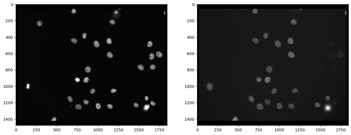
首先，我们需要分离通道（了解更多）。之后，我们实际上可以看到，并非所有用Cy3标记的细胞（通道0）也被eGFP标记（通道1）：

# extract channels
channel_cy3 = raw_image[...,0]
channel_egfp = raw_image[...,1]

# visualize
fig, axs = plt.subplots(1, 2, figsize=(15,15))
axs[0].imshow(channel_cy3, cmap='gray')
axs[1].imshow(channel_egfp, cmap='gray')

<matplotlib.image.AxesImage at 0x1dac7328970>

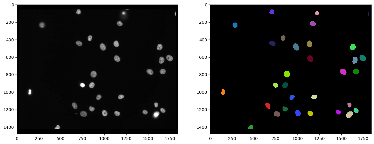
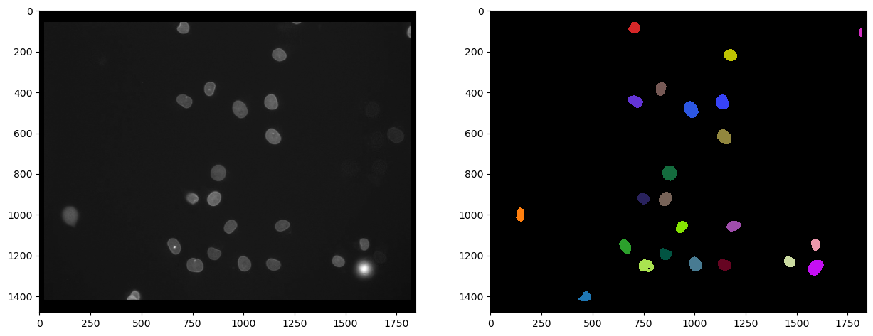
细胞核分割

由于染色在Cy3通道标记了细胞核，因此在这个通道中分割细胞核并随后测量另一个通道的强度是合理的。我们使用Voronoi-Otsu-Labeling进行分割，因为这是一种快速直接的方法。

# segmentation
nuclei_cy3 = cle.voronoi_otsu_labeling(channel_cy3, spot_sigma=20)

# visualize
fig, axs = plt.subplots(1, 2, figsize=(15,15))
cle.imshow(channel_cy3, plot=axs[0], color_map="gray")
cle.imshow(nuclei_cy3, plot=axs[1], labels=True)

C:\Users\rober\miniconda3\envs\bio39\lib\site-packages\pyclesperanto_prototype\_tier9\_imshow.py:46: UserWarning: The imshow parameter color_map is deprecated. Use colormap instead.
  warnings.warn("The imshow parameter color_map is deprecated. Use colormap instead.")

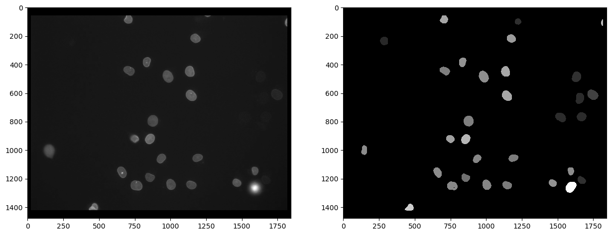
首先，我们可以测量第二个通道（标记为eGFP）的强度，并在参数图像中可视化该测量结果。在这样的参数图像中，细胞核内的所有像素都具有相同的值，在这种情况下是细胞的平均强度。

intensity_map = cle.mean_intensity_map(channel_egfp, nuclei_cy3)

# visualize
fig, axs = plt.subplots(1, 2, figsize=(15,15))
cle.imshow(channel_egfp, plot=axs[0], color_map="gray")
cle.imshow(intensity_map, plot=axs[1], color_map="gray")

C:\Users\rober\miniconda3\envs\bio39\lib\site-packages\pyclesperanto_prototype\_tier9\_imshow.py:46: UserWarning: The imshow parameter color_map is deprecated. Use colormap instead.
  warnings.warn("The imshow parameter color_map is deprecated. Use colormap instead.")

从这样的参数图像中，我们可以提取强度值并将它们放入一个向量中。这个列表中的第一项值为0，对应于背景的强度，在参数图像中为0。

intensity_vector = cle.read_intensities_from_map(nuclei_cy3, intensity_map)
intensity_vector

cle.array([[  0.        80.875854  23.529799 118.17817   80.730255  95.55177
   72.84752   92.34759   78.84362   85.400444 105.108025  65.06639
   73.69295   77.40091   81.48371   77.12868   96.58209   95.94536
   70.883995  89.70502   72.01046   27.257877  84.460075  25.49711
   80.69057  147.49736   28.112642  25.167627  28.448263  25.31705
   38.072815 108.81613 ]], dtype=float32)

顺便说一下，还有另一种直接获得平均强度的方法，即通过测量包括位置和形状在内的细胞核的所有属性。这些统计数据可以进一步作为pandas DataFrame处理。

statistics = cle.statistics_of_background_and_labelled_pixels(channel_egfp, nuclei_cy3)

statistics_df = pd.DataFrame(statistics)
statistics_df.head()

	label	original_label	bbox_min_x	bbox_min_y	bbox_min_z	bbox_max_x	bbox_max_y	bbox_max_z	bbox_width	bbox_height	...	centroid_z	sum_distance_to_centroid	mean_distance_to_centroid	sum_distance_to_mass_center	mean_distance_to_mass_center	standard_deviation_intensity	max_distance_to_centroid	max_distance_to_mass_center	mean_max_distance_to_centroid_ratio	mean_max_distance_to_mass_center_ratio
0	1	0	0.0	0.0	0.0	1841.0	1477.0	0.0	1842.0	1478.0	...	0.0	1.683849e+09	640.648682	1.683884e+09	640.661682	8.487288	1187.033203	1187.743164	1.852861	1.853932
1	2	1	127.0	967.0	0.0	167.0	1033.0	0.0	41.0	67.0	...	0.0	4.128044e+04	18.704323	4.128327e+04	18.705606	4.734930	34.280727	34.338104	1.832770	1.835712
2	3	2	259.0	205.0	0.0	314.0	265.0	0.0	56.0	61.0	...	0.0	5.392080e+04	19.715099	5.393993e+04	19.722092	1.663603	32.079941	31.469477	1.627176	1.595646
3	4	3	432.0	1377.0	0.0	492.0	1423.0	0.0	61.0	47.0	...	0.0	3.630314e+04	17.769527	3.636823e+04	17.801388	24.842560	36.856213	36.085457	2.074125	2.027115
4	5	4	631.0	1123.0	0.0	690.0	1194.0	0.0	60.0	72.0	...	0.0	6.753254e+04	21.686750	6.755171e+04	21.692907	17.358543	38.805695	38.417568	1.789373	1.770974

5 rows × 37 columns

然后可以从表格统计数据中提取强度向量。注意：在这种情况下，背景强度不是0，因为我们直接从原始图像中读取它。

intensity_vector2 = statistics['mean_intensity']
intensity_vector2

array([ 20.829758,  80.875854,  23.529799, 118.17817 ,  80.730255,
        95.55177 ,  72.84752 ,  92.34759 ,  78.84362 ,  85.400444,
       105.108025,  65.06639 ,  73.69295 ,  77.40091 ,  81.48371 ,
        77.12868 ,  96.58209 ,  95.94536 ,  70.883995,  89.70502 ,
        72.01046 ,  27.257877,  84.460075,  25.49711 ,  80.69057 ,
       147.49736 ,  28.112642,  25.167627,  28.448263,  25.31705 ,
        38.072815, 108.81613 ], dtype=float32)

为了概览平均强度测量，我们可以使用matplotlib绘制直方图。我们忽略第一个元素，因为它对应于背景强度。

plt.hist(intensity_vector2[1:])

(array([ 7.,  1.,  0.,  4., 10.,  5.,  2.,  1.,  0.,  1.]),
 array([ 23.52979851,  35.92655563,  48.32331085,  60.72006607,
         73.11682129,  85.51358032,  97.91033936, 110.30709076,
        122.70384979, 135.1006012 , 147.49736023]),
 <BarContainer object of 10 artists>)

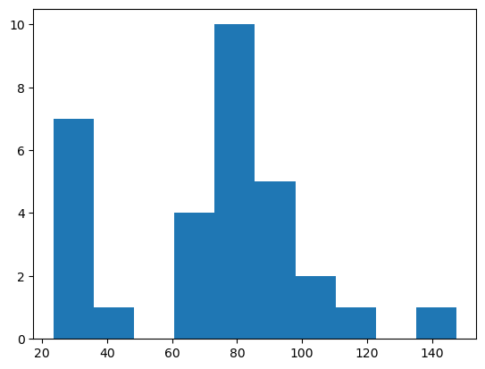
从这样的直方图中，我们可以得出结论，强度高于50的对象是阳性的。

选择高于给定强度阈值的标签

接下来，我们生成一个新的标签图像，其中包含强度 > 50的细胞核。注意，上述所有提取强度向量的步骤对此并不是必需的。我们这样做只是为了对一个好的强度阈值有一个概念。

以下标签图像显示了在Cy3通道中分割的细胞核，这些细胞核在eGFP通道中具有高强度。

intensity_threshold = 50

nuclei_with_high_intensity_egfg = cle.exclude_labels_with_map_values_within_range(intensity_map, nuclei_cy3, maximum_value_range=intensity_threshold)
intensity_map = cle.mean_intensity_map(channel_egfp, nuclei_cy3)

# visualize
fig, axs = plt.subplots(1, 2, figsize=(15,15))
cle.imshow(channel_egfp, plot=axs[0], color_map="gray")
cle.imshow(nuclei_with_high_intensity_egfg, plot=axs[1], labels=True)

C:\Users\rober\miniconda3\envs\bio39\lib\site-packages\pyclesperanto_prototype\_tier9\_imshow.py:46: UserWarning: The imshow parameter color_map is deprecated. Use colormap instead.
  warnings.warn("The imshow parameter color_map is deprecated. Use colormap instead.")

我们还可以通过确定标签图像中的最大强度来计算这些细胞的数量：

number_of_double_positives = nuclei_with_high_intensity_egfg.max()
print("同时表达Cy3和eGFP的细胞核数量", number_of_double_positives)

Number of Cy3 nuclei that also express eGFP 23.0

参考资料

我们使用的一些函数可能不太常见。因此，我们可以添加它们的文档以供参考。

print(cle.voronoi_otsu_labeling.__doc__)

Labels objects directly from grey-value images.

    The two sigma parameters allow tuning the segmentation result. Under the hood,
    this filter applies two Gaussian blurs, spot detection, Otsu-thresholding [2] and Voronoi-labeling [3]. The
    thresholded binary image is flooded using the Voronoi tesselation approach starting from the found local maxima.

    Notes
    -----
    * This operation assumes input images are isotropic.

    Parameters
    ----------
    source : Image
        Input grey-value image
    label_image_destination : Image, optional
        Output image
    spot_sigma : float, optional
        controls how close detected cells can be
    outline_sigma : float, optional
        controls how precise segmented objects are outlined.
    
    Returns
    -------
    label_image_destination
    
    Examples
    --------
    >>> import pyclesperanto_prototype as cle
    >>> cle.voronoi_otsu_labeling(source, label_image_destination, 10, 2)
    
    References
    ----------
    .. [1] https://clij.github.io/clij2-docs/reference_voronoiOtsuLabeling
    .. [2] https://ieeexplore.ieee.org/document/4310076
    .. [3] https://en.wikipedia.org/wiki/Voronoi_diagram
    

print(cle.mean_intensity_map.__doc__)

Takes an image and a corresponding label map, determines the mean 
    intensity per label and replaces every label with the that number.
    
    This results in a parametric image expressing mean object intensity. 
    
    Parameters
    ----------
    source : Image
    label_map : Image
    destination : Image, optional
    
    Returns
    -------
    destination
    
    References
    ----------
    .. [1] https://clij.github.io/clij2-docs/reference_meanIntensityMap
    

print(cle.read_intensities_from_map.__doc__)

Takes a label image and a parametric image to read parametric values from the labels positions.
    The read intensity values are stored in a new vector.

    Note: This will only work if all labels have number of voxels == 1 or if all pixels in each label have the same value.

    Parameters
    ----------
    labels: Image
    map_image: Image
    values_destination: Image, optional
        1d vector with length == number of labels + 1

    Returns
    -------
    values_destination, Image:
        vector of intensity values with 0th element corresponding to background and subsequent entries corresponding to
        the intensity in the given labeled object
    

print(cle.statistics_of_background_and_labelled_pixels.__doc__)

Determines bounding box, area (in pixels/voxels), min, max and mean 
    intensity of background and labelled objects in a label map and corresponding
    pixels in the original image.
    
    Instead of a label map, you can also use a binary image as a binary image is a 
    label map with just one label.
    
    This method is executed on the CPU and not on the GPU/OpenCL device. 
    
    Parameters
    ----------
    source : Image
    labelmap : Image

    Returns
    -------
    Dictionary of measurements
    
    References
    ----------
    .. [1] https://clij.github.io/clij2-docs/reference_statisticsOfBackgroundAndLabelledPixels
    

print(cle.exclude_labels_with_map_values_within_range.__doc__)

This operation removes labels from a labelmap and renumbers the
    remaining labels.

    Notes
    -----
    * Values of all pixels in a label each must be identical.

    Parameters
    ----------
    values_map : Image
    label_map_input : Image
    label_map_destination : Image, optional
    minimum_value_range : Number, optional
    maximum_value_range : Number, optional

    Returns
    -------
    label_map_destination

    References
    ----------
    .. [1] https://clij.github.io/clij2-docs/reference_excludeLabelsWithValuesWithinRange