测量标签边界的强度

在某些应用中，测量标签边界的强度是合理的。例如，为了测量显示细胞核包膜的图像中的信号强度，可以对细胞核进行分割，识别它们的边界，然后在那里测量强度。

import numpy as np
from skimage.io import imread, imshow
import pyclesperanto_prototype as cle
from cellpose import models, io
from skimage import measure
import matplotlib.pyplot as plt

2022-02-24 10:05:10,405 [INFO] WRITING LOG OUTPUT TO C:\Users\rober\.cellpose\run.log

示例数据集

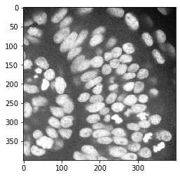
在这个例子中，我们加载了一张显示斑马鱼眼睛的图像，由德累斯顿马克斯·普朗克分子细胞生物学与遗传学研究所Norden实验室的Mauricio Rocha Martins提供。

multichannel_image = imread("../../data/zfish_eye.tif")
multichannel_image.shape

(1024, 1024, 3)

cropped_image = multichannel_image[200:600, 500:900]

nuclei_channel = cropped_image[:,:,0]

cle.imshow(nuclei_channel)

图像分割

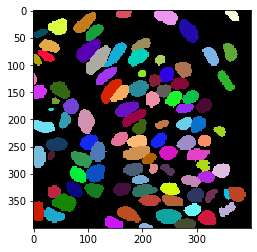
首先，我们使用cellpose来分割细胞

# load cellpose model
model = models.Cellpose(gpu=False, model_type='nuclei')

# apply model
channels = [0,0] # This means we are processing single channel greyscale images.
label_image, flows, styles, diams = model.eval(nuclei_channel, diameter=None, channels=channels)

# show result
cle.imshow(label_image, labels=True)

2022-02-24 10:05:10,623 [INFO] >>>> using CPU
2022-02-24 10:05:10,675 [INFO] ~~~ ESTIMATING CELL DIAMETER(S) ~~~
2022-02-24 10:05:13,858 [INFO] estimated cell diameter(s) in 3.18 sec
2022-02-24 10:05:13,859 [INFO] >>> diameter(s) = 
2022-02-24 10:05:13,860 [INFO] [ 29.64 ]
2022-02-24 10:05:13,860 [INFO] ~~~ FINDING MASKS ~~~
2022-02-24 10:05:18,649 [INFO] >>>> TOTAL TIME 7.97 sec

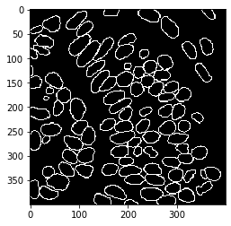
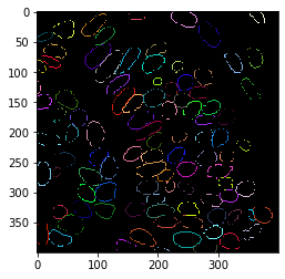
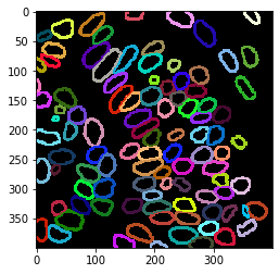
标记标签边界上的像素

接下来，我们将提取分割后的细胞核的轮廓。

binary_borders = cle.detect_label_edges(label_image)

labeled_borders = binary_borders * label_image

cle.imshow(label_image, labels=True)
cle.imshow(binary_borders)
cle.imshow(labeled_borders, labels=True)

扩张轮廓

我们稍微扩展轮廓以获得更稳健的测量。

extended_outlines = cle.dilate_labels(labeled_borders, radius=2)

cle.imshow(extended_outlines, labels=True)

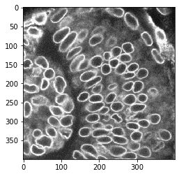
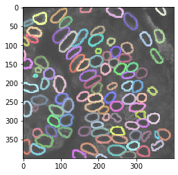
叠加可视化

使用这个细胞核轮廓的标签图像，我们可以测量核包膜中的强度。

nuclear_envelope_channel = cropped_image[:,:,2]

cle.imshow(nuclear_envelope_channel)

cle.imshow(nuclear_envelope_channel, alpha=0.5, continue_drawing=True)
cle.imshow(extended_outlines, alpha=0.5, labels=True)

标签强度统计

使用正确的强度和标签图像可以测量图像中的强度。

stats = cle.statistics_of_labelled_pixels(nuclear_envelope_channel, extended_outlines)

stats["mean_intensity"]

array([35529.4  , 32835.07 , 36713.887, 37146.348, 49462.39 , 36392.6  ,
       37998.375, 48974.945, 31805.87 , 50451.793, 41006.047, 50854.016,
       36167.547, 41332.32 , 37815.766, 35121.38 , 43859.945, 40292.875,
       31583.992, 38933.57 , 32297.547, 39140.766, 37072.31 , 45990.57 ,
       39800.613, 37804.99 , 39092.43 , 39510.848, 40534.81 , 42057.293,
       44815.844, 42855.754, 38408.246, 41257.594, 37996.895, 38568.465,
       42331.266, 34748.973, 44219.844, 41986.086, 38606.215, 39008.094,
       36411.05 , 48155.797, 43781.97 , 38315.12 , 36048.39 , 37739.277,
       46268.816, 35808.32 , 37388.312, 37682.21 , 42932.72 , 38168.293,
       40489.73 , 43073.066, 40973.285, 40975.246, 39292.848, 38555.766,
       38219.785, 40054.242, 37356.87 , 45014.8  , 37211.668, 47025.47 ,
       30218.678, 33988.027, 37338.41 , 38500.85 , 38546.777, 40611.742,
       40391.453, 41024.46 , 37840.246, 41342.793, 39329.625, 43311.016,
       37829.074, 39949.82 , 39316.496, 40966.48 , 34066.7  , 34929.863,
       40356.445, 31959.607, 39480.855, 39194.027, 46274.582, 31316.648,
       37623.61 , 40962.016, 39203.37 , 45368.703, 37830.832, 35296.93 ,
       37756.1  , 39108.93 , 40739.543], dtype=float32)

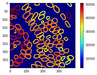
参数图

这些测量结果也可以使用参数图进行可视化

intensity_map = cle.mean_intensity_map(nuclear_envelope_channel, extended_outlines)
cle.imshow(intensity_map, min_display_intensity=3000, colorbar=True, colormap="jet")

练习

测量并可视化细胞核通道中标签边界的强度。