使用APOC和基于SimpleITK的特征进行对象分类#
对象分类可能涉及提取自定义特征。我们通过使用napari-simpleitk-image-processing中可用的基于SimpleITK的特征来模拟这种场景,并训练一个APOC 表格行分类器。
另请参见
from skimage.io import imread
from pyclesperanto_prototype import imshow, replace_intensities
from skimage.filters import threshold_otsu
from skimage.measure import label, regionprops
import numpy as np
import pandas as pd
import matplotlib.pyplot as plt
from napari_simpleitk_image_processing import label_statistics
import apoc
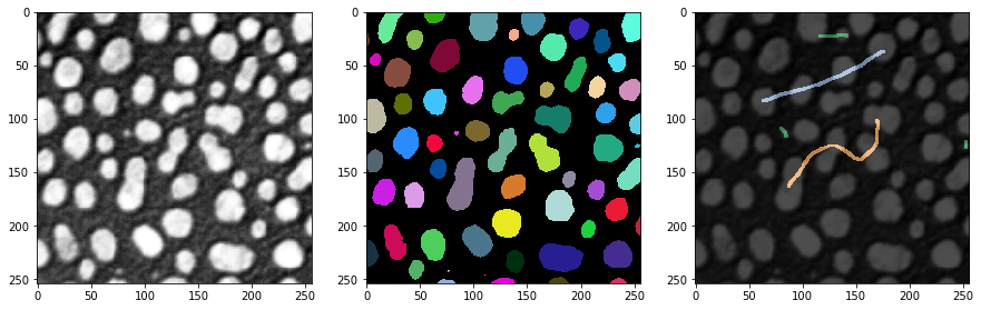
我们的起点是一张图像、一个标签图像和一些基础事实注释。注释也是一个标签图像,其中用户只是用不同强度(类别)的线条穿过小对象、大对象和细长对象进行绘制。
# load and label data
image = imread('../../data/blobs.tif')
labels = label(image > threshold_otsu(image))
annotation = imread('../../data/label_annotation.tif')

# visualize
fig, ax = plt.subplots(1,3, figsize=(15,15))
imshow(image, plot=ax[0])
imshow(labels, plot=ax[1], labels=True)
imshow(image, plot=ax[2], continue_drawing=True)
imshow(annotation, plot=ax[2], alpha=0.7, labels=True)
特征提取#
根据对象属性进行分类的第一步是特征提取。我们将使用可脚本化的napari插件napari-simpleitk-image-processing来完成这个任务。
statistics = label_statistics(image, labels, None, True, True, True, True, True, True)

statistics_table = pd.DataFrame(statistics)
statistics_table
| label | maximum | mean | median | minimum | sigma | sum | variance | bbox_0 | bbox_1 | ... | number_of_pixels_on_border | perimeter | perimeter_on_border | perimeter_on_border_ratio | principal_axes0 | principal_axes1 | principal_axes2 | principal_axes3 | principal_moments0 | principal_moments1 | |
|---|---|---|---|---|---|---|---|---|---|---|---|---|---|---|---|---|---|---|---|---|---|
| 0 | 1 | 232.0 | 190.854503 | 200.0 | 128.0 | 30.304925 | 82640.0 | 918.388504 | 10 | 0 | ... | 17 | 89.196525 | 17.0 | 0.190590 | 0.902586 | 0.430509 | -0.430509 | 0.902586 | 17.680049 | 76.376232 |
| 1 | 2 | 224.0 | 179.286486 | 184.0 | 128.0 | 21.883314 | 33168.0 | 478.879436 | 53 | 0 | ... | 21 | 53.456120 | 21.0 | 0.392846 | -0.051890 | -0.998653 | 0.998653 | -0.051890 | 8.708186 | 27.723954 |
| 2 | 3 | 248.0 | 205.617021 | 208.0 | 128.0 | 29.380812 | 135296.0 | 863.232099 | 95 | 0 | ... | 23 | 93.409370 | 23.0 | 0.246228 | 0.988608 | 0.150515 | -0.150515 | 0.988608 | 49.978765 | 57.049896 |
| 3 | 4 | 248.0 | 217.327189 | 232.0 | 128.0 | 36.061134 | 94320.0 | 1300.405402 | 144 | 0 | ... | 19 | 75.558902 | 19.0 | 0.251459 | 0.870813 | 0.491615 | -0.491615 | 0.870813 | 33.246984 | 37.624111 |
| 4 | 5 | 248.0 | 212.142558 | 224.0 | 128.0 | 29.904270 | 101192.0 | 894.265349 | 237 | 0 | ... | 39 | 82.127941 | 40.0 | 0.487045 | 0.998987 | 0.045005 | -0.045005 | 0.998987 | 24.584386 | 60.694273 |
| ... | ... | ... | ... | ... | ... | ... | ... | ... | ... | ... | ... | ... | ... | ... | ... | ... | ... | ... | ... | ... | ... |
| 59 | 60 | 128.0 | 128.000000 | 128.0 | 128.0 | 0.000000 | 128.0 | 0.000000 | 110 | 246 | ... | 0 | 2.681517 | 0.0 | 0.000000 | 1.000000 | 0.000000 | 0.000000 | 1.000000 | 0.000000 | 0.000000 |
| 60 | 61 | 248.0 | 183.407407 | 176.0 | 128.0 | 34.682048 | 14856.0 | 1202.844444 | 170 | 248 | ... | 19 | 41.294008 | 19.0 | 0.460115 | -0.005203 | -0.999986 | 0.999986 | -0.005203 | 2.190911 | 21.525901 |
| 61 | 62 | 216.0 | 181.511111 | 184.0 | 128.0 | 25.599001 | 16336.0 | 655.308864 | 116 | 249 | ... | 23 | 48.093086 | 23.0 | 0.478239 | -0.023708 | -0.999719 | 0.999719 | -0.023708 | 1.801689 | 31.523372 |
| 62 | 63 | 248.0 | 188.377358 | 184.0 | 128.0 | 38.799398 | 9984.0 | 1505.393324 | 227 | 249 | ... | 16 | 34.264893 | 16.0 | 0.466950 | 0.004852 | -0.999988 | 0.999988 | 0.004852 | 1.603845 | 13.711214 |
| 63 | 64 | 224.0 | 172.897959 | 176.0 | 128.0 | 28.743293 | 8472.0 | 826.176871 | 66 | 250 | ... | 17 | 35.375614 | 17.0 | 0.480557 | 0.022491 | -0.999747 | 0.999747 | 0.022491 | 0.923304 | 18.334505 |
64 rows × 33 columns
statistics_table.columns
Index(['label', 'maximum', 'mean', 'median', 'minimum', 'sigma', 'sum',
       'variance', 'bbox_0', 'bbox_1', 'bbox_2', 'bbox_3', 'centroid_0',
       'centroid_1', 'elongation', 'feret_diameter', 'flatness', 'roundness',
       'equivalent_ellipsoid_diameter_0', 'equivalent_ellipsoid_diameter_1',
       'equivalent_spherical_perimeter', 'equivalent_spherical_radius',
       'number_of_pixels', 'number_of_pixels_on_border', 'perimeter',
       'perimeter_on_border', 'perimeter_on_border_ratio', 'principal_axes0',
       'principal_axes1', 'principal_axes2', 'principal_axes3',
       'principal_moments0', 'principal_moments1'],
      dtype='object')
table = statistics_table[['number_of_pixels','elongation']]
table
| number_of_pixels | elongation | |
|---|---|---|
| 0 | 433 | 2.078439 |
| 1 | 185 | 1.784283 |
| 2 | 658 | 1.068402 |
| 3 | 434 | 1.063793 |
| 4 | 477 | 1.571246 |
| ... | ... | ... |
| 59 | 1 | 0.000000 |
| 60 | 81 | 3.134500 |
| 61 | 90 | 4.182889 |
| 62 | 53 | 2.923862 |
| 63 | 49 | 4.456175 |
64 rows × 2 columns
我们还从基础事实注释中读取每个标记对象的最大强度。这些值将用于训练分类器。值为0的条目对应于未被注释的对象。
annotation_stats = regionprops(labels, intensity_image=annotation)

annotated_classes = np.asarray([s.max_intensity for s in annotation_stats])
print(annotated_classes)
[0. 0. 2. 0. 0. 0. 2. 0. 0. 0. 3. 0. 0. 0. 3. 0. 0. 3. 0. 0. 0. 3. 0. 0.
 0. 0. 1. 0. 0. 0. 1. 2. 1. 0. 0. 2. 0. 1. 0. 0. 0. 0. 0. 0. 0. 0. 0. 0.
 0. 0. 0. 0. 0. 0. 0. 0. 0. 0. 0. 0. 0. 0. 0. 0.]
分类器训练#
接下来,我们可以训练随机森林分类器。它需要表格训练数据和一个基础事实向量。
classifier_filename = 'table_row_classifier.cl'

classifier = apoc.TableRowClassifier(opencl_filename=classifier_filename, max_depth=2, num_ensembles=10)
classifier.train(table, annotated_classes)
预测#
要将分类器应用于整个数据集或任何其他数据集,我们需要确保数据格式相同。如果我们分析的是训练所用的同一数据集,这是很简单的。
predicted_classes = classifier.predict(table)
predicted_classes
array([1, 1, 2, 3, 3, 3, 2, 3, 2, 1, 3, 3, 3, 2, 3, 1, 3, 3, 3, 3, 3, 3,
       1, 3, 3, 3, 3, 1, 3, 3, 1, 2, 1, 2, 2, 3, 3, 1, 1, 3, 3, 3, 3, 2,
       3, 2, 3, 2, 1, 3, 1, 3, 3, 1, 3, 3, 3, 3, 1, 2, 1, 1, 1, 1],
      dtype=uint32)
为了文档记录的目的,我们可以将注释类别和预测类别保存到我们的表格中。注意:我们在训练之后这样做,因为否则例如列
table
| number_of_pixels | elongation | |
|---|---|---|
| 0 | 433 | 2.078439 |
| 1 | 185 | 1.784283 |
| 2 | 658 | 1.068402 |
| 3 | 434 | 1.063793 |
| 4 | 477 | 1.571246 |
| ... | ... | ... |
| 59 | 1 | 0.000000 |
| 60 | 81 | 3.134500 |
| 61 | 90 | 4.182889 |
| 62 | 53 | 2.923862 |
| 63 | 49 | 4.456175 |
64 rows × 2 columns
table['annotated_class'] = annotated_classes
table['predicted_class'] = predicted_classes
table
/var/folders/p1/6svzckgd1y5906pfgm71fvmr0000gn/T/ipykernel_4463/2818530951.py:1: SettingWithCopyWarning:
A value is trying to be set on a copy of a slice from a DataFrame.
Try using .loc[row_indexer,col_indexer] = value instead

See the caveats in the documentation: https://pandas.pydata.org/pandas-docs/stable/user_guide/indexing.html#returning-a-view-versus-a-copy
  table['annotated_class'] = annotated_classes
/var/folders/p1/6svzckgd1y5906pfgm71fvmr0000gn/T/ipykernel_4463/2818530951.py:2: SettingWithCopyWarning:
A value is trying to be set on a copy of a slice from a DataFrame.
Try using .loc[row_indexer,col_indexer] = value instead

See the caveats in the documentation: https://pandas.pydata.org/pandas-docs/stable/user_guide/indexing.html#returning-a-view-versus-a-copy
  table['predicted_class'] = predicted_classes
| number_of_pixels | elongation | annotated_class | predicted_class | |
|---|---|---|---|---|
| 0 | 433 | 2.078439 | 0.0 | 1 |
| 1 | 185 | 1.784283 | 0.0 | 1 |
| 2 | 658 | 1.068402 | 2.0 | 2 |
| 3 | 434 | 1.063793 | 0.0 | 3 |
| 4 | 477 | 1.571246 | 0.0 | 3 |
| ... | ... | ... | ... | ... |
| 59 | 1 | 0.000000 | 0.0 | 2 |
| 60 | 81 | 3.134500 | 0.0 | 1 |
| 61 | 90 | 4.182889 | 0.0 | 1 |
| 62 | 53 | 2.923862 | 0.0 | 1 |
| 63 | 49 | 4.456175 | 0.0 | 1 |
64 rows × 4 columns
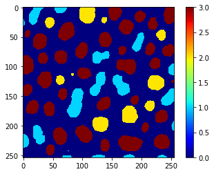
此外,我们可以使用相同的向量来使用replace_intensities生成一个class_image。背景和测量中有NaN的对象在该图像中的值为0。
# we add a 0 for the class of background at the beginning
predicted_classes_with_background = [0] + predicted_classes.tolist()
print(predicted_classes_with_background)
[0, 1, 1, 2, 3, 3, 3, 2, 3, 2, 1, 3, 3, 3, 2, 3, 1, 3, 3, 3, 3, 3, 3, 1, 3, 3, 3, 3, 1, 3, 3, 1, 2, 1, 2, 2, 3, 3, 1, 1, 3, 3, 3, 3, 2, 3, 2, 3, 2, 1, 3, 1, 3, 3, 1, 3, 3, 3, 3, 1, 2, 1, 1, 1, 1]
class_image = replace_intensities(labels, predicted_classes_with_background)
imshow(class_image, colorbar=True, colormap='jet', min_display_intensity=0)