滤波概览#
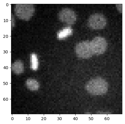
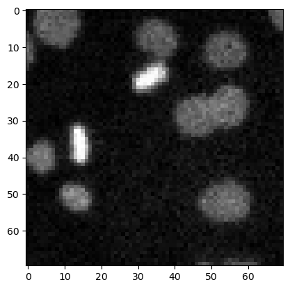
在本笔记本中,我们使用细胞核示例图像演示一些更典型的滤波器。
import numpy as np

import matplotlib.pyplot as plt
from skimage.io import imread
from skimage import data
from skimage import filters
from skimage import morphology
from scipy.ndimage import convolve, gaussian_laplace
import stackview
image3 = imread('../../data/mitosis_mod.tif').astype(float)

plt.imshow(image3, cmap='gray')
<matplotlib.image.AxesImage at 0x12d1b7ce940>
去噪#
用于图像去噪的常见滤波器包括均值滤波器、中值滤波器和高斯滤波器。
denoised_mean = filters.rank.mean(image3.astype(np.uint8), morphology.disk(1))

plt.imshow(denoised_mean, cmap='gray')
<matplotlib.image.AxesImage at 0x12d1ba2df10>
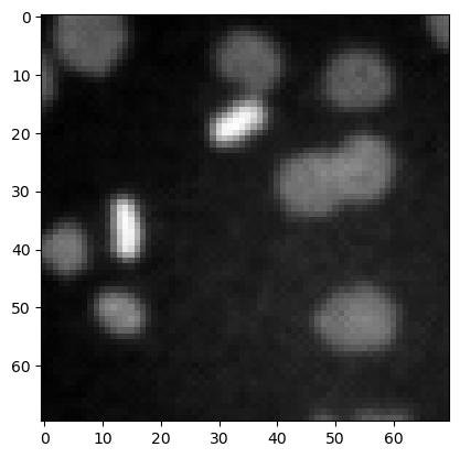
denoised_median = filters.median(image3, morphology.disk(1))

plt.imshow(denoised_median, cmap='gray')
<matplotlib.image.AxesImage at 0x12d1b8ef340>

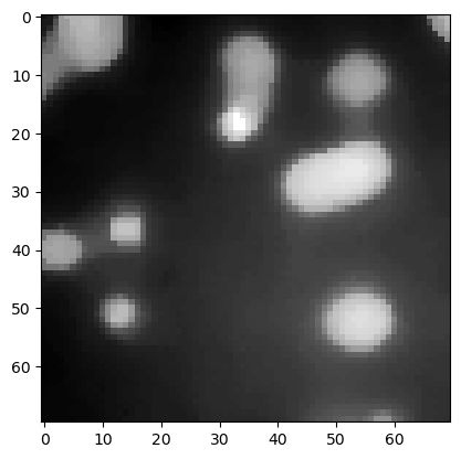
denoised_median2 = filters.median(image3, morphology.disk(5))

plt.imshow(denoised_median2, cmap='gray')
<matplotlib.image.AxesImage at 0x12d1b96bb20>
denoised_gaussian = filters.gaussian(image3, sigma=1)

plt.imshow(denoised_gaussian, cmap='gray')
<matplotlib.image.AxesImage at 0x12d1bbbb880>

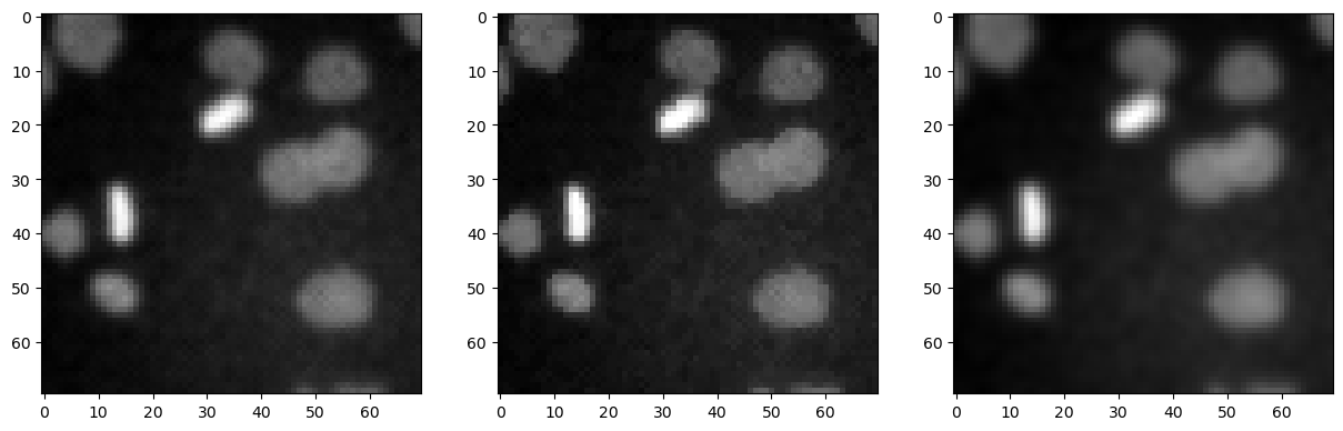
我们还可以使用matplotlib将这些图像并排显示。
fig, axes = plt.subplots(1,3, figsize=(15,15))

axes[0].imshow(denoised_mean, cmap='gray')
axes[1].imshow(denoised_median, cmap='gray')
axes[2].imshow(denoised_gaussian, cmap='gray')
<matplotlib.image.AxesImage at 0x12d1bae6d60>
顶帽滤波 / 背景去除#
top_hat = morphology.white_tophat(image3, morphology.disk(15))

plt.imshow(top_hat, cmap='gray')
<matplotlib.image.AxesImage at 0x12d1d549c10>
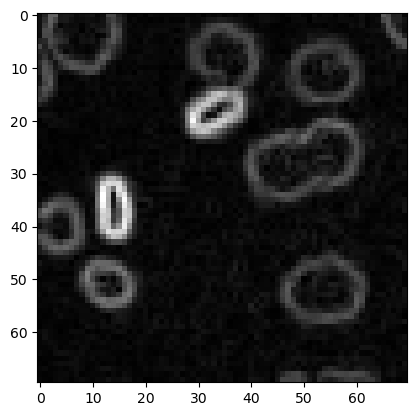
边缘检测#
sobel = filters.sobel(image3)

plt.imshow(sobel, cmap='gray')
<matplotlib.image.AxesImage at 0x12d1ccc6bb0>
练习#
应用不同半径的顶帽滤波器,并将它们并排显示。