定量图像分析

定量图像分析#

在对图像中的对象进行分割和标记之后，我们可以测量这些对象的属性。

另请参阅

在进行测量之前，我们需要一个image和相应的label_image。因此，我们回顾一下过滤、阈值处理和标记：

from skimage.io import imread
from skimage import filters
from skimage import measure
from pyclesperanto_prototype import imshow
import pandas as pd 
import numpy as np

# load image
image = imread("../../data/blobs.tif")

# denoising
blurred_image = filters.gaussian(image, sigma=1)

# binarization
threshold = filters.threshold_otsu(blurred_image)
thresholded_image = blurred_image >= threshold

# labeling
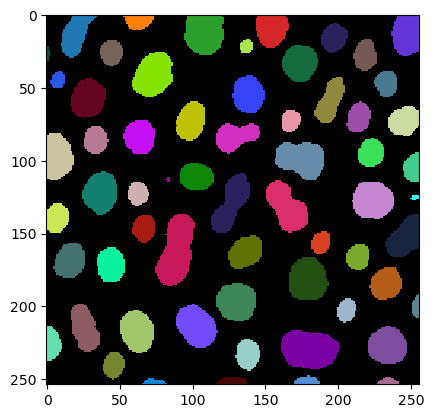
label_image = measure.label(thresholded_image)

# visualization
imshow(label_image, labels=True)

../_images/5257573298d6a444b6a34d09506d6cf9a10aab208bce52c927a91ea6491b20ee.png

测量 / 区域属性#

为了读取区域的属性，我们使用regionprops函数：

# analyse objects
properties = measure.regionprops(label_image, intensity_image=image)

结果以RegionProps对象的形式存储，这些对象不是很直观：

properties[0:5]

[<skimage.measure._regionprops.RegionProperties at 0x1c272b8f8e0>,
 <skimage.measure._regionprops.RegionProperties at 0x1c26d278af0>,
 <skimage.measure._regionprops.RegionProperties at 0x1c26d2784c0>,
 <skimage.measure._regionprops.RegionProperties at 0x1c26d278b20>,
 <skimage.measure._regionprops.RegionProperties at 0x1c26d278b80>]

如果你想知道我们测量了哪些属性：它们列在measure.regionprops函数的文档中。基本上，我们现在有一个变量properties，它包含40个不同的特征。但我们只对其中的一小部分感兴趣。

因此，我们可以将测量结果重新组织成一个包含我们感兴趣的特征数组的字典：

statistics = {
    'area':       [p.area               for p in properties],
    'mean':       [p.mean_intensity     for p in properties],
    'major_axis': [p.major_axis_length  for p in properties],
    'minor_axis': [p.minor_axis_length for p in properties]
}

读取这些数组字典并不是很方便。为此，我们引入了数据科学家常用的pandas DataFrames。”DataFrames”只是Python中用于”表格”的另一个术语。

df = pd.DataFrame(statistics)
df

	area	mean	major_axis	minor_axis
0	429	191.440559	34.779230	16.654732
1	183	179.846995	20.950530	11.755645
2	658	205.604863	30.198484	28.282790
3	433	217.515012	24.508791	23.079220
4	472	213.033898	31.084766	19.681190
...	...	...	...	...
57	213	184.525822	18.753879	14.468993
58	79	184.810127	18.287489	5.762488
59	88	182.727273	21.673692	5.389867
60	52	189.538462	14.335104	5.047883
61	48	173.833333	16.925660	3.831678

62 rows × 4 columns

你还可以通过计算自己的指标来添加自定义列，例如aspect_ratio：

df['aspect_ratio'] = [p.major_axis_length / p.minor_axis_length for p in properties]
df

	area	mean	major_axis	minor_axis	aspect_ratio
0	429	191.440559	34.779230	16.654732	2.088249
1	183	179.846995	20.950530	11.755645	1.782168
2	658	205.604863	30.198484	28.282790	1.067734
3	433	217.515012	24.508791	23.079220	1.061942
4	472	213.033898	31.084766	19.681190	1.579415
...	...	...	...	...	...
57	213	184.525822	18.753879	14.468993	1.296143
58	79	184.810127	18.287489	5.762488	3.173540
59	88	182.727273	21.673692	5.389867	4.021193
60	52	189.538462	14.335104	5.047883	2.839825
61	48	173.833333	16.925660	3.831678	4.417297

62 rows × 5 columns

这些数据框可以方便地保存到磁盘：

df.to_csv("blobs_analysis.csv")

此外，我们可以使用numpy来测量statistics表中的属性。例如，平均面积：

# measure mean area
np.mean(df['area'])

355.3709677419355

练习#

分析加载的斑点image。

其中有多少个对象？

最大的对象有多大？

图像的平均值和标准差是多少？

分割对象面积的平均值和标准差是多少？

定量图像分析

Contents

定量图像分析#

测量 / 区域属性#

练习#