Diferenciación de núcleos según la intensidad de la señal

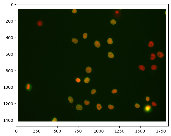
Una tarea común en el análisis de bioimágenes es diferenciar células según su expresión de señal. En este ejemplo, tomamos una imagen de dos canales de núcleos que expresan Cy3 y eGFP. Visualmente, podemos ver fácilmente que algunos núcleos que expresan Cy3 también expresan eGFP, mientras que otros no. Este notebook demuestra cómo diferenciar núcleos segmentados en un canal según la intensidad en el otro canal.

import pyclesperanto_prototype as cle
import numpy as np
from skimage.io import imread, imshow
import matplotlib.pyplot as plt
import pandas as pd

cle.get_device()

<Intel(R) Iris(R) Xe Graphics on Platform: Intel(R) OpenCL HD Graphics (1 refs)>

Estamos utilizando un conjunto de datos publicado por Heriche et al. con licencia CC BY 4.0 disponible en el Image Data Resource.

# load file
raw_image = imread('../../data/plate1_1_013 [Well 5, Field 1 (Spot 5)].png')

# visualize
imshow(raw_image)

<matplotlib.image.AxesImage at 0x1dac72d7c40>

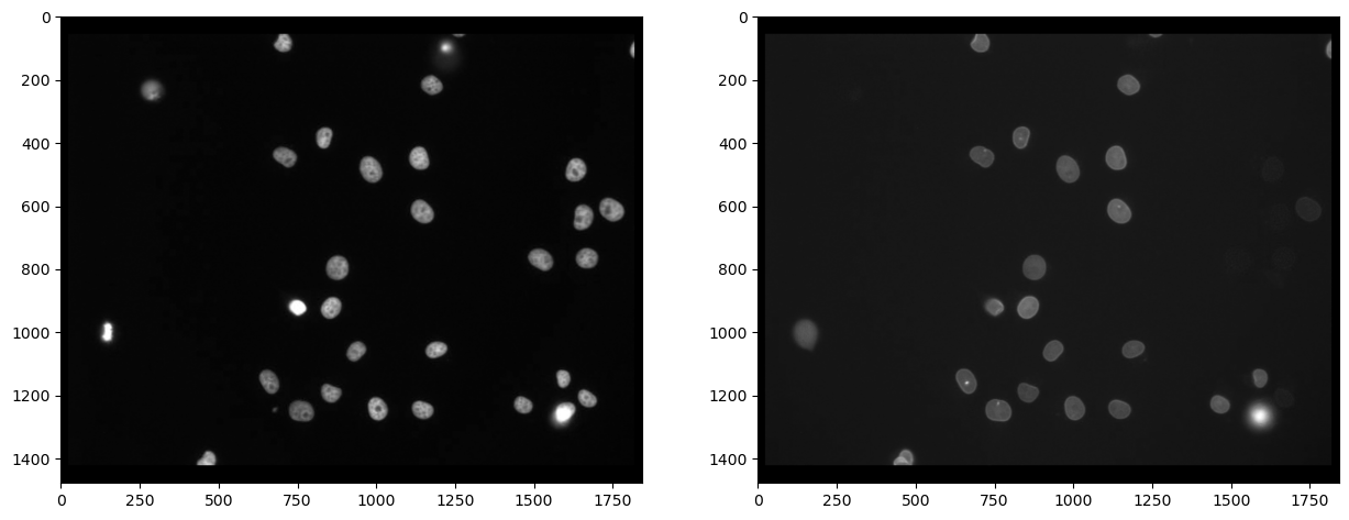
Primero, necesitamos separar los canales (leer más). Después de eso, realmente podemos ver que no todas las células marcadas con Cy3 (canal 0) también están marcadas con eGFP (canal 1):

# extract channels
channel_cy3 = raw_image[...,0]
channel_egfp = raw_image[...,1]

# visualize
fig, axs = plt.subplots(1, 2, figsize=(15,15))
axs[0].imshow(channel_cy3, cmap='gray')
axs[1].imshow(channel_egfp, cmap='gray')

<matplotlib.image.AxesImage at 0x1dac7328970>

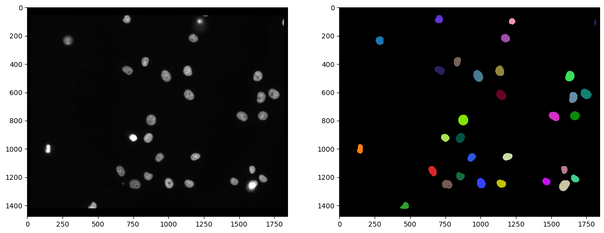
Segmentación de núcleos

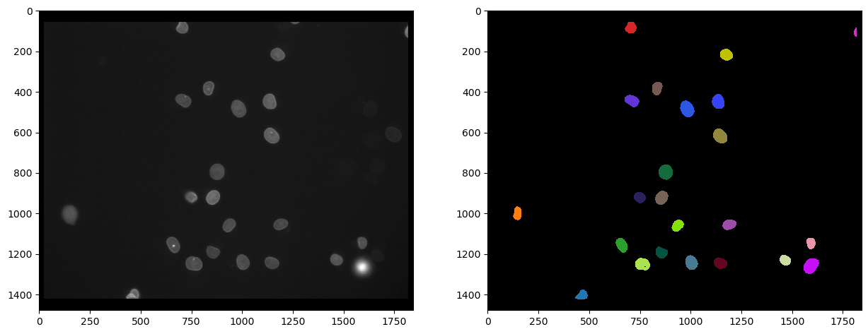
Como la tinción marca los núcleos en el canal Cy3, es razonable segmentar los núcleos en este canal y después medir la intensidad en el otro canal. Usamos Voronoi-Otsu-Labeling para la segmentación porque es un enfoque rápido y directo.

# segmentation
nuclei_cy3 = cle.voronoi_otsu_labeling(channel_cy3, spot_sigma=20)

# visualize
fig, axs = plt.subplots(1, 2, figsize=(15,15))
cle.imshow(channel_cy3, plot=axs[0], color_map="gray")
cle.imshow(nuclei_cy3, plot=axs[1], labels=True)

C:\Users\rober\miniconda3\envs\bio39\lib\site-packages\pyclesperanto_prototype\_tier9\_imshow.py:46: UserWarning: The imshow parameter color_map is deprecated. Use colormap instead.
  warnings.warn("The imshow parameter color_map is deprecated. Use colormap instead.")

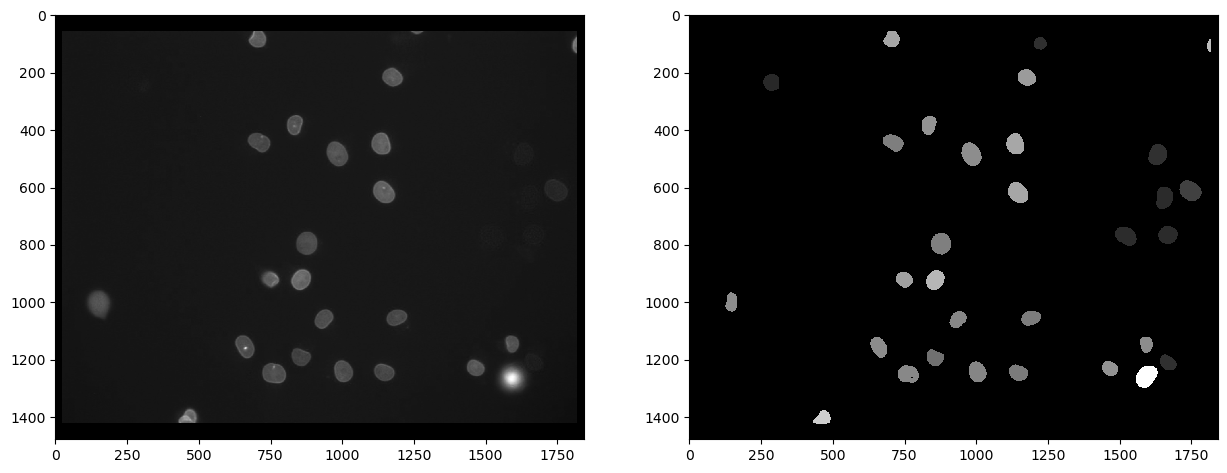
En primer lugar, podemos medir la intensidad en el segundo canal, marcado con eGFP y visualizar esa medición en una imagen paramétrica. En tal imagen paramétrica, todos los píxeles dentro de un núcleo tienen el mismo valor, en este caso la intensidad media promedio de la célula.

intensity_map = cle.mean_intensity_map(channel_egfp, nuclei_cy3)

# visualize
fig, axs = plt.subplots(1, 2, figsize=(15,15))
cle.imshow(channel_egfp, plot=axs[0], color_map="gray")
cle.imshow(intensity_map, plot=axs[1], color_map="gray")

C:\Users\rober\miniconda3\envs\bio39\lib\site-packages\pyclesperanto_prototype\_tier9\_imshow.py:46: UserWarning: The imshow parameter color_map is deprecated. Use colormap instead.
  warnings.warn("The imshow parameter color_map is deprecated. Use colormap instead.")

A partir de tal imagen paramétrica, podemos recuperar los valores de intensidad y obtenerlos en un vector. El primer elemento de esta lista tiene valor 0 y corresponde a la intensidad del fondo, que es 0 en la imagen paramétrica.

intensity_vector = cle.read_intensities_from_map(nuclei_cy3, intensity_map)
intensity_vector

cle.array([[  0.        80.875854  23.529799 118.17817   80.730255  95.55177
   72.84752   92.34759   78.84362   85.400444 105.108025  65.06639
   73.69295   77.40091   81.48371   77.12868   96.58209   95.94536
   70.883995  89.70502   72.01046   27.257877  84.460075  25.49711
   80.69057  147.49736   28.112642  25.167627  28.448263  25.31705
   38.072815 108.81613 ]], dtype=float32)

Por cierto, también hay una forma alternativa de llegar a las intensidades medias directamente, midiendo todas las propiedades de los núcleos, incluyendo posición y forma. Las estadísticas pueden procesarse adicionalmente como un DataFrame de pandas.

statistics = cle.statistics_of_background_and_labelled_pixels(channel_egfp, nuclei_cy3)

statistics_df = pd.DataFrame(statistics)
statistics_df.head()

	label	original_label	bbox_min_x	bbox_min_y	bbox_min_z	bbox_max_x	bbox_max_y	bbox_max_z	bbox_width	bbox_height	...	centroid_z	sum_distance_to_centroid	mean_distance_to_centroid	sum_distance_to_mass_center	mean_distance_to_mass_center	standard_deviation_intensity	max_distance_to_centroid	max_distance_to_mass_center	mean_max_distance_to_centroid_ratio	mean_max_distance_to_mass_center_ratio
0	1	0	0.0	0.0	0.0	1841.0	1477.0	0.0	1842.0	1478.0	...	0.0	1.683849e+09	640.648682	1.683884e+09	640.661682	8.487288	1187.033203	1187.743164	1.852861	1.853932
1	2	1	127.0	967.0	0.0	167.0	1033.0	0.0	41.0	67.0	...	0.0	4.128044e+04	18.704323	4.128327e+04	18.705606	4.734930	34.280727	34.338104	1.832770	1.835712
2	3	2	259.0	205.0	0.0	314.0	265.0	0.0	56.0	61.0	...	0.0	5.392080e+04	19.715099	5.393993e+04	19.722092	1.663603	32.079941	31.469477	1.627176	1.595646
3	4	3	432.0	1377.0	0.0	492.0	1423.0	0.0	61.0	47.0	...	0.0	3.630314e+04	17.769527	3.636823e+04	17.801388	24.842560	36.856213	36.085457	2.074125	2.027115
4	5	4	631.0	1123.0	0.0	690.0	1194.0	0.0	60.0	72.0	...	0.0	6.753254e+04	21.686750	6.755171e+04	21.692907	17.358543	38.805695	38.417568	1.789373	1.770974

5 rows × 37 columns

El vector de intensidad puede entonces recuperarse de las estadísticas tabulares. Nota: En este caso, la intensidad del fondo no es 0, porque la estábamos leyendo directamente de la imagen original.

intensity_vector2 = statistics['mean_intensity']
intensity_vector2

array([ 20.829758,  80.875854,  23.529799, 118.17817 ,  80.730255,
        95.55177 ,  72.84752 ,  92.34759 ,  78.84362 ,  85.400444,
       105.108025,  65.06639 ,  73.69295 ,  77.40091 ,  81.48371 ,
        77.12868 ,  96.58209 ,  95.94536 ,  70.883995,  89.70502 ,
        72.01046 ,  27.257877,  84.460075,  25.49711 ,  80.69057 ,
       147.49736 ,  28.112642,  25.167627,  28.448263,  25.31705 ,
        38.072815, 108.81613 ], dtype=float32)

Para obtener una visión general de la medición de intensidad media, podemos usar matplotlib para trazar un histograma. Ignoramos el primer elemento, porque corresponde a la intensidad del fondo.

plt.hist(intensity_vector2[1:])

(array([ 7.,  1.,  0.,  4., 10.,  5.,  2.,  1.,  0.,  1.]),
 array([ 23.52979851,  35.92655563,  48.32331085,  60.72006607,
         73.11682129,  85.51358032,  97.91033936, 110.30709076,
        122.70384979, 135.1006012 , 147.49736023]),
 <BarContainer object of 10 artists>)

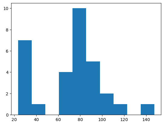
A partir de tal histograma, podríamos concluir que los objetos con intensidad superior a 50 son positivos.

Selección de etiquetas por encima de un umbral de intensidad dado

A continuación, generamos una nueva imagen de etiquetas con los núcleos que tienen una intensidad > 50. Nota, todos los pasos anteriores para extraer el vector de intensidad no son necesarios para esto. Solo lo hicimos para tener una idea de un buen umbral de intensidad.

La siguiente imagen de etiquetas muestra los núcleos segmentados en el canal Cy3 que tienen una alta intensidad en el canal eGFP.

intensity_threshold = 50

nuclei_with_high_intensity_egfg = cle.exclude_labels_with_map_values_within_range(intensity_map, nuclei_cy3, maximum_value_range=intensity_threshold)
intensity_map = cle.mean_intensity_map(channel_egfp, nuclei_cy3)

# visualize
fig, axs = plt.subplots(1, 2, figsize=(15,15))
cle.imshow(channel_egfp, plot=axs[0], color_map="gray")
cle.imshow(nuclei_with_high_intensity_egfg, plot=axs[1], labels=True)

C:\Users\rober\miniconda3\envs\bio39\lib\site-packages\pyclesperanto_prototype\_tier9\_imshow.py:46: UserWarning: The imshow parameter color_map is deprecated. Use colormap instead.
  warnings.warn("The imshow parameter color_map is deprecated. Use colormap instead.")

Y también podemos contarlos determinando la intensidad máxima en la imagen de etiquetas:

number_of_double_positives = nuclei_with_high_intensity_egfg.max()
print("Número de núcleos Cy3 que también expresan eGFP", number_of_double_positives)

Number of Cy3 nuclei that also express eGFP 23.0

Referencias

Algunas de las funciones que usamos pueden ser poco comunes. Por lo tanto, podemos agregar su documentación como referencia.

print(cle.voronoi_otsu_labeling.__doc__)

Labels objects directly from grey-value images.

    The two sigma parameters allow tuning the segmentation result. Under the hood,
    this filter applies two Gaussian blurs, spot detection, Otsu-thresholding [2] and Voronoi-labeling [3]. The
    thresholded binary image is flooded using the Voronoi tesselation approach starting from the found local maxima.

    Notes
    -----
    * This operation assumes input images are isotropic.

    Parameters
    ----------
    source : Image
        Input grey-value image
    label_image_destination : Image, optional
        Output image
    spot_sigma : float, optional
        controls how close detected cells can be
    outline_sigma : float, optional
        controls how precise segmented objects are outlined.
    
    Returns
    -------
    label_image_destination
    
    Examples
    --------
    >>> import pyclesperanto_prototype as cle
    >>> cle.voronoi_otsu_labeling(source, label_image_destination, 10, 2)
    
    References
    ----------
    .. [1] https://clij.github.io/clij2-docs/reference_voronoiOtsuLabeling
    .. [2] https://ieeexplore.ieee.org/document/4310076
    .. [3] https://en.wikipedia.org/wiki/Voronoi_diagram
    

print(cle.mean_intensity_map.__doc__)

Takes an image and a corresponding label map, determines the mean 
    intensity per label and replaces every label with the that number.
    
    This results in a parametric image expressing mean object intensity. 
    
    Parameters
    ----------
    source : Image
    label_map : Image
    destination : Image, optional
    
    Returns
    -------
    destination
    
    References
    ----------
    .. [1] https://clij.github.io/clij2-docs/reference_meanIntensityMap
    

print(cle.read_intensities_from_map.__doc__)

Takes a label image and a parametric image to read parametric values from the labels positions.
    The read intensity values are stored in a new vector.

    Note: This will only work if all labels have number of voxels == 1 or if all pixels in each label have the same value.

    Parameters
    ----------
    labels: Image
    map_image: Image
    values_destination: Image, optional
        1d vector with length == number of labels + 1

    Returns
    -------
    values_destination, Image:
        vector of intensity values with 0th element corresponding to background and subsequent entries corresponding to
        the intensity in the given labeled object
    

print(cle.statistics_of_background_and_labelled_pixels.__doc__)

Determines bounding box, area (in pixels/voxels), min, max and mean 
    intensity of background and labelled objects in a label map and corresponding
    pixels in the original image.
    
    Instead of a label map, you can also use a binary image as a binary image is a 
    label map with just one label.
    
    This method is executed on the CPU and not on the GPU/OpenCL device. 
    
    Parameters
    ----------
    source : Image
    labelmap : Image

    Returns
    -------
    Dictionary of measurements
    
    References
    ----------
    .. [1] https://clij.github.io/clij2-docs/reference_statisticsOfBackgroundAndLabelledPixels
    

print(cle.exclude_labels_with_map_values_within_range.__doc__)

This operation removes labels from a labelmap and renumbers the
    remaining labels.

    Notes
    -----
    * Values of all pixels in a label each must be identical.

    Parameters
    ----------
    values_map : Image
    label_map_input : Image
    label_map_destination : Image, optional
    minimum_value_range : Number, optional
    maximum_value_range : Number, optional

    Returns
    -------
    label_map_destination

    References
    ----------
    .. [1] https://clij.github.io/clij2-docs/reference_excludeLabelsWithValuesWithinRange