Clasificación de objetos con APOC y características basadas en SimpleITK#
La clasificación de objetos puede implicar la extracción de características personalizadas. Simulamos este escenario utilizando características basadas en SimpleITK disponibles en napari-simpleitk-image-processing y entrenamos un clasificador de filas de tabla de APOC.
Ver también
from skimage.io import imread
from pyclesperanto_prototype import imshow, replace_intensities
from skimage.filters import threshold_otsu
from skimage.measure import label, regionprops
import numpy as np
import pandas as pd
import matplotlib.pyplot as plt
from napari_simpleitk_image_processing import label_statistics
import apoc
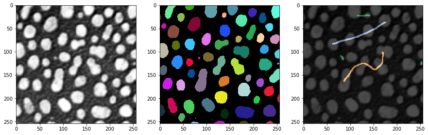
Nuestro punto de partida son una imagen, una imagen de etiquetas y algunas anotaciones de referencia. La anotación también es una imagen de etiquetas donde el usuario simplemente dibujó líneas con diferentes intensidades (clases) a través de objetos pequeños, objetos grandes y objetos alargados.
# load and label data
image = imread('../../data/blobs.tif')
labels = label(image > threshold_otsu(image))
annotation = imread('../../data/label_annotation.tif')

# visualize
fig, ax = plt.subplots(1,3, figsize=(15,15))
imshow(image, plot=ax[0])
imshow(labels, plot=ax[1], labels=True)
imshow(image, plot=ax[2], continue_drawing=True)
imshow(annotation, plot=ax[2], alpha=0.7, labels=True)
Extracción de características#
El primer paso para clasificar objetos según sus propiedades es la extracción de características. Usaremos el complemento napari programable napari-simpleitk-image-processing para eso.
statistics = label_statistics(image, labels, None, True, True, True, True, True, True)

statistics_table = pd.DataFrame(statistics)
statistics_table
| label | maximum | mean | median | minimum | sigma | sum | variance | bbox_0 | bbox_1 | ... | number_of_pixels_on_border | perimeter | perimeter_on_border | perimeter_on_border_ratio | principal_axes0 | principal_axes1 | principal_axes2 | principal_axes3 | principal_moments0 | principal_moments1 | |
|---|---|---|---|---|---|---|---|---|---|---|---|---|---|---|---|---|---|---|---|---|---|
| 0 | 1 | 232.0 | 190.854503 | 200.0 | 128.0 | 30.304925 | 82640.0 | 918.388504 | 10 | 0 | ... | 17 | 89.196525 | 17.0 | 0.190590 | 0.902586 | 0.430509 | -0.430509 | 0.902586 | 17.680049 | 76.376232 |
| 1 | 2 | 224.0 | 179.286486 | 184.0 | 128.0 | 21.883314 | 33168.0 | 478.879436 | 53 | 0 | ... | 21 | 53.456120 | 21.0 | 0.392846 | -0.051890 | -0.998653 | 0.998653 | -0.051890 | 8.708186 | 27.723954 |
| 2 | 3 | 248.0 | 205.617021 | 208.0 | 128.0 | 29.380812 | 135296.0 | 863.232099 | 95 | 0 | ... | 23 | 93.409370 | 23.0 | 0.246228 | 0.988608 | 0.150515 | -0.150515 | 0.988608 | 49.978765 | 57.049896 |
| 3 | 4 | 248.0 | 217.327189 | 232.0 | 128.0 | 36.061134 | 94320.0 | 1300.405402 | 144 | 0 | ... | 19 | 75.558902 | 19.0 | 0.251459 | 0.870813 | 0.491615 | -0.491615 | 0.870813 | 33.246984 | 37.624111 |
| 4 | 5 | 248.0 | 212.142558 | 224.0 | 128.0 | 29.904270 | 101192.0 | 894.265349 | 237 | 0 | ... | 39 | 82.127941 | 40.0 | 0.487045 | 0.998987 | 0.045005 | -0.045005 | 0.998987 | 24.584386 | 60.694273 |
| ... | ... | ... | ... | ... | ... | ... | ... | ... | ... | ... | ... | ... | ... | ... | ... | ... | ... | ... | ... | ... | ... |
| 59 | 60 | 128.0 | 128.000000 | 128.0 | 128.0 | 0.000000 | 128.0 | 0.000000 | 110 | 246 | ... | 0 | 2.681517 | 0.0 | 0.000000 | 1.000000 | 0.000000 | 0.000000 | 1.000000 | 0.000000 | 0.000000 |
| 60 | 61 | 248.0 | 183.407407 | 176.0 | 128.0 | 34.682048 | 14856.0 | 1202.844444 | 170 | 248 | ... | 19 | 41.294008 | 19.0 | 0.460115 | -0.005203 | -0.999986 | 0.999986 | -0.005203 | 2.190911 | 21.525901 |
| 61 | 62 | 216.0 | 181.511111 | 184.0 | 128.0 | 25.599001 | 16336.0 | 655.308864 | 116 | 249 | ... | 23 | 48.093086 | 23.0 | 0.478239 | -0.023708 | -0.999719 | 0.999719 | -0.023708 | 1.801689 | 31.523372 |
| 62 | 63 | 248.0 | 188.377358 | 184.0 | 128.0 | 38.799398 | 9984.0 | 1505.393324 | 227 | 249 | ... | 16 | 34.264893 | 16.0 | 0.466950 | 0.004852 | -0.999988 | 0.999988 | 0.004852 | 1.603845 | 13.711214 |
| 63 | 64 | 224.0 | 172.897959 | 176.0 | 128.0 | 28.743293 | 8472.0 | 826.176871 | 66 | 250 | ... | 17 | 35.375614 | 17.0 | 0.480557 | 0.022491 | -0.999747 | 0.999747 | 0.022491 | 0.923304 | 18.334505 |
64 rows × 33 columns
statistics_table.columns
Index(['label', 'maximum', 'mean', 'median', 'minimum', 'sigma', 'sum',
       'variance', 'bbox_0', 'bbox_1', 'bbox_2', 'bbox_3', 'centroid_0',
       'centroid_1', 'elongation', 'feret_diameter', 'flatness', 'roundness',
       'equivalent_ellipsoid_diameter_0', 'equivalent_ellipsoid_diameter_1',
       'equivalent_spherical_perimeter', 'equivalent_spherical_radius',
       'number_of_pixels', 'number_of_pixels_on_border', 'perimeter',
       'perimeter_on_border', 'perimeter_on_border_ratio', 'principal_axes0',
       'principal_axes1', 'principal_axes2', 'principal_axes3',
       'principal_moments0', 'principal_moments1'],
      dtype='object')
table = statistics_table[['number_of_pixels','elongation']]
table
| number_of_pixels | elongation | |
|---|---|---|
| 0 | 433 | 2.078439 |
| 1 | 185 | 1.784283 |
| 2 | 658 | 1.068402 |
| 3 | 434 | 1.063793 |
| 4 | 477 | 1.571246 |
| ... | ... | ... |
| 59 | 1 | 0.000000 |
| 60 | 81 | 3.134500 |
| 61 | 90 | 4.182889 |
| 62 | 53 | 2.923862 |
| 63 | 49 | 4.456175 |
64 rows × 2 columns
También leemos la intensidad máxima de cada objeto etiquetado de la anotación de referencia. Estos valores servirán para entrenar el clasificador. Las entradas de 0 corresponden a objetos que no han sido anotados.
annotation_stats = regionprops(labels, intensity_image=annotation)

annotated_classes = np.asarray([s.max_intensity for s in annotation_stats])
print(annotated_classes)
[0. 0. 2. 0. 0. 0. 2. 0. 0. 0. 3. 0. 0. 0. 3. 0. 0. 3. 0. 0. 0. 3. 0. 0.
 0. 0. 1. 0. 0. 0. 1. 2. 1. 0. 0. 2. 0. 1. 0. 0. 0. 0. 0. 0. 0. 0. 0. 0.
 0. 0. 0. 0. 0. 0. 0. 0. 0. 0. 0. 0. 0. 0. 0. 0.]
Entrenamiento del Clasificador#
A continuación, podemos entrenar el Clasificador de Bosque Aleatorio. Necesita datos de entrenamiento en forma de tabla y un vector de verdad de referencia.
classifier_filename = 'table_row_classifier.cl'

classifier = apoc.TableRowClassifier(opencl_filename=classifier_filename, max_depth=2, num_ensembles=10)
classifier.train(table, annotated_classes)
Predicción#
Para aplicar un clasificador a todo el conjunto de datos, o cualquier otro conjunto de datos, debemos asegurarnos de que los datos estén en el mismo formato. Esto es trivial en caso de que analicemos el mismo conjunto de datos en el que entrenamos.
predicted_classes = classifier.predict(table)
predicted_classes
array([1, 1, 2, 3, 3, 3, 2, 3, 2, 1, 3, 3, 3, 2, 3, 1, 3, 3, 3, 3, 3, 3,
       1, 3, 3, 3, 3, 1, 3, 3, 1, 2, 1, 2, 2, 3, 3, 1, 1, 3, 3, 3, 3, 2,
       3, 2, 3, 2, 1, 3, 1, 3, 3, 1, 3, 3, 3, 3, 1, 2, 1, 1, 1, 1],
      dtype=uint32)
Con fines de documentación, podemos guardar la clase anotada y la clase predicha en nuestra tabla. Nota: Estamos haciendo esto después del entrenamiento, porque de lo contrario, por ejemplo, la columna
table
| number_of_pixels | elongation | |
|---|---|---|
| 0 | 433 | 2.078439 |
| 1 | 185 | 1.784283 |
| 2 | 658 | 1.068402 |
| 3 | 434 | 1.063793 |
| 4 | 477 | 1.571246 |
| ... | ... | ... |
| 59 | 1 | 0.000000 |
| 60 | 81 | 3.134500 |
| 61 | 90 | 4.182889 |
| 62 | 53 | 2.923862 |
| 63 | 49 | 4.456175 |
64 rows × 2 columns
table['annotated_class'] = annotated_classes
table['predicted_class'] = predicted_classes
table
/var/folders/p1/6svzckgd1y5906pfgm71fvmr0000gn/T/ipykernel_4463/2818530951.py:1: SettingWithCopyWarning:
A value is trying to be set on a copy of a slice from a DataFrame.
Try using .loc[row_indexer,col_indexer] = value instead

See the caveats in the documentation: https://pandas.pydata.org/pandas-docs/stable/user_guide/indexing.html#returning-a-view-versus-a-copy
  table['annotated_class'] = annotated_classes
/var/folders/p1/6svzckgd1y5906pfgm71fvmr0000gn/T/ipykernel_4463/2818530951.py:2: SettingWithCopyWarning:
A value is trying to be set on a copy of a slice from a DataFrame.
Try using .loc[row_indexer,col_indexer] = value instead

See the caveats in the documentation: https://pandas.pydata.org/pandas-docs/stable/user_guide/indexing.html#returning-a-view-versus-a-copy
  table['predicted_class'] = predicted_classes
| number_of_pixels | elongation | annotated_class | predicted_class | |
|---|---|---|---|---|
| 0 | 433 | 2.078439 | 0.0 | 1 |
| 1 | 185 | 1.784283 | 0.0 | 1 |
| 2 | 658 | 1.068402 | 2.0 | 2 |
| 3 | 434 | 1.063793 | 0.0 | 3 |
| 4 | 477 | 1.571246 | 0.0 | 3 |
| ... | ... | ... | ... | ... |
| 59 | 1 | 0.000000 | 0.0 | 2 |
| 60 | 81 | 3.134500 | 0.0 | 1 |
| 61 | 90 | 4.182889 | 0.0 | 1 |
| 62 | 53 | 2.923862 | 0.0 | 1 |
| 63 | 49 | 4.456175 | 0.0 | 1 |
64 rows × 4 columns
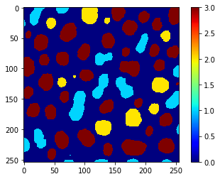
Además, podemos usar el mismo vector para utilizar replace_intensities para generar una class_image. El fondo y los objetos con NaNs en las mediciones tendrán valor 0 en esa imagen.
# we add a 0 for the class of background at the beginning
predicted_classes_with_background = [0] + predicted_classes.tolist()
print(predicted_classes_with_background)
[0, 1, 1, 2, 3, 3, 3, 2, 3, 2, 1, 3, 3, 3, 2, 3, 1, 3, 3, 3, 3, 3, 3, 1, 3, 3, 3, 3, 1, 3, 3, 1, 2, 1, 2, 2, 3, 3, 1, 1, 3, 3, 3, 3, 2, 3, 2, 3, 2, 1, 3, 1, 3, 3, 1, 3, 3, 3, 3, 1, 2, 1, 1, 1, 1]
class_image = replace_intensities(labels, predicted_classes_with_background)
imshow(class_image, colorbar=True, colormap='jet', min_display_intensity=0)