Aperçu des filtres#
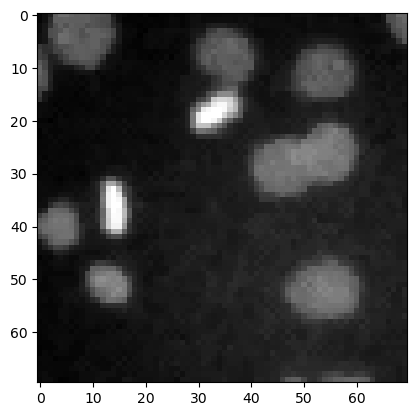
Dans ce notebook, nous démontrons quelques filtres plus typiques en utilisant l’image d’exemple des noyaux.
import numpy as np

import matplotlib.pyplot as plt
from skimage.io import imread
from skimage import data
from skimage import filters
from skimage import morphology
from scipy.ndimage import convolve, gaussian_laplace
import stackview
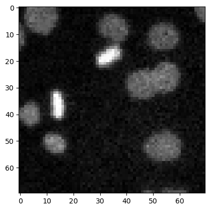
image3 = imread('../../data/mitosis_mod.tif').astype(float)

plt.imshow(image3, cmap='gray')
<matplotlib.image.AxesImage at 0x12d1b7ce940>

Débruitage#
Les filtres couramment utilisés pour débruiter les images sont le filtre moyen, le filtre médian et le filtre gaussien.
denoised_mean = filters.rank.mean(image3.astype(np.uint8), morphology.disk(1))

plt.imshow(denoised_mean, cmap='gray')
<matplotlib.image.AxesImage at 0x12d1ba2df10>

denoised_median = filters.median(image3, morphology.disk(1))

plt.imshow(denoised_median, cmap='gray')
<matplotlib.image.AxesImage at 0x12d1b8ef340>
denoised_median2 = filters.median(image3, morphology.disk(5))

plt.imshow(denoised_median2, cmap='gray')
<matplotlib.image.AxesImage at 0x12d1b96bb20>
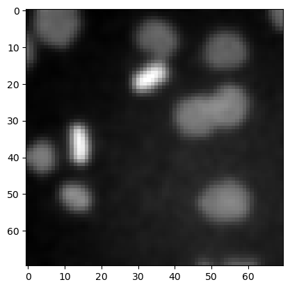
denoised_gaussian = filters.gaussian(image3, sigma=1)

plt.imshow(denoised_gaussian, cmap='gray')
<matplotlib.image.AxesImage at 0x12d1bbbb880>
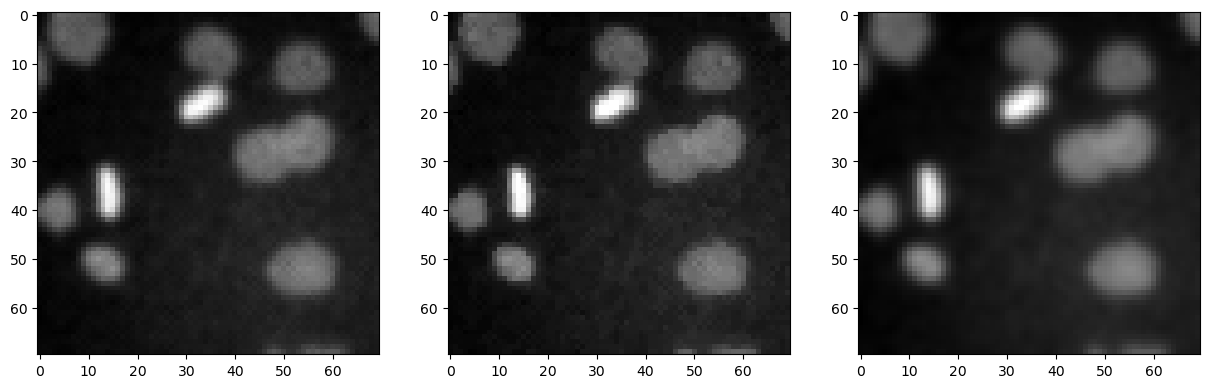
Nous pouvons également afficher ces images côte à côte en utilisant matplotlib.
fig, axes = plt.subplots(1,3, figsize=(15,15))

axes[0].imshow(denoised_mean, cmap='gray')
axes[1].imshow(denoised_median, cmap='gray')
axes[2].imshow(denoised_gaussian, cmap='gray')
<matplotlib.image.AxesImage at 0x12d1bae6d60>
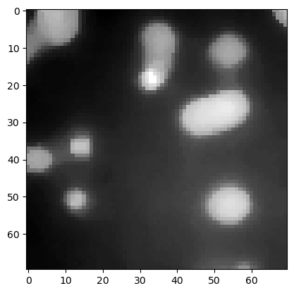
Filtrage Top-hat / suppression du fond#
top_hat = morphology.white_tophat(image3, morphology.disk(15))

plt.imshow(top_hat, cmap='gray')
<matplotlib.image.AxesImage at 0x12d1d549c10>
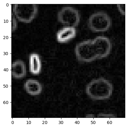
Détection de contours#
sobel = filters.sobel(image3)

plt.imshow(sobel, cmap='gray')
<matplotlib.image.AxesImage at 0x12d1ccc6bb0>
Exercice#
Appliquez différents rayons pour le filtre top-hat et affichez-les côte à côte.