Image Processing with scikit-image

In this notebook, we’ll explore basic image processing techniques using the scikit-image library. We’ll learn how to load, display, and manipulate images using various filters and transformations.

First, let’s import the necessary libraries. We’ll use scikit-image for image processing and matplotlib for displaying images.

import numpy as np
from skimage import data, filters, color
import matplotlib.pyplot as plt

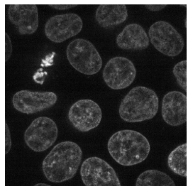
Now, let’s load a sample image from scikit-image’s data module. We’ll use the ‘cells3d’ image for this example.

image = data.cells3d()[30, 1]  # Select a specific slice from the 3D image
plt.imshow(image, cmap='gray')
plt.axis('off')
plt.show()

Downloading file 'data/cells3d.tif' from 'https://gitlab.com/scikit-image/data/-/raw/2cdc5ce89b334d28f06a58c9f0ca21aa6992a5ba/cells3d.tif' to '/home/runner/.cache/scikit-image/0.21.0'.

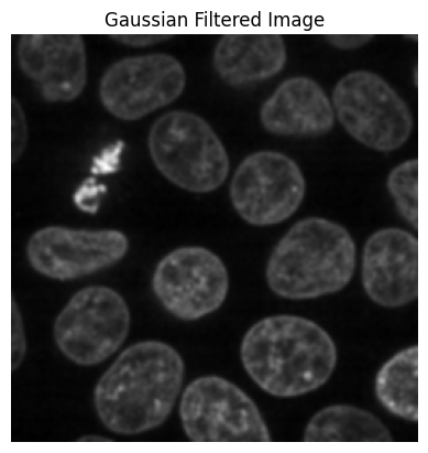
Let’s apply a Gaussian filter to smooth the image. This filter reduces noise and blurs the image slightly.

gaussian_image = filters.gaussian(image, sigma=1)
plt.imshow(gaussian_image, cmap='gray')
plt.axis('off')
plt.title('Gaussian Filtered Image')
plt.show()

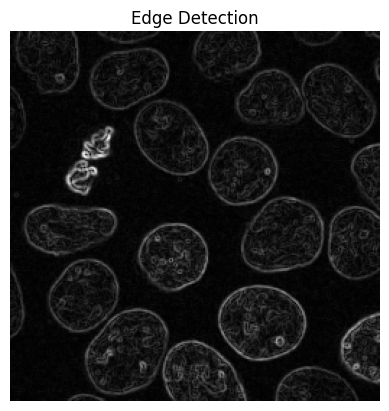
Next, we’ll apply edge detection using the Sobel filter. This filter highlights edges in the image.

edges = filters.sobel(image)
plt.imshow(edges, cmap='gray')
plt.axis('off')
plt.title('Edge Detection')
plt.show()

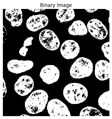
Now, let’s threshold the image to create a binary image. This separates the foreground from the background.

threshold_value = filters.threshold_otsu(image)
binary_image = image > threshold_value
plt.imshow(binary_image, cmap='gray')
plt.axis('off')
plt.title('Binary Image')
plt.show()

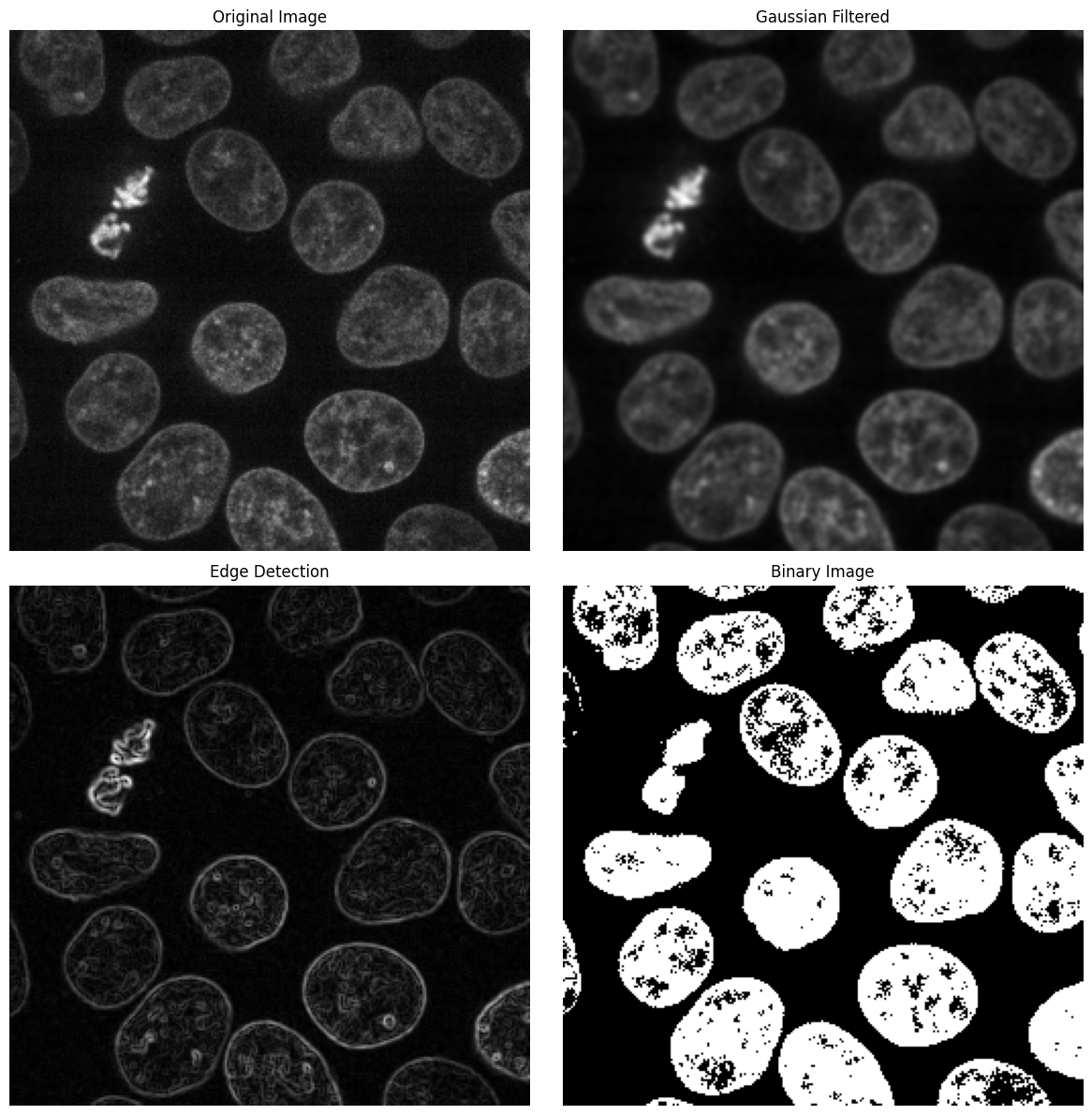
Finally, let’s compare the original image with the processed versions side by side.

fig, axes = plt.subplots(2, 2, figsize=(12, 12))
axes[0, 0].imshow(image, cmap='gray')
axes[0, 0].set_title('Original Image')
axes[0, 1].imshow(gaussian_image, cmap='gray')
axes[0, 1].set_title('Gaussian Filtered')
axes[1, 0].imshow(edges, cmap='gray')
axes[1, 0].set_title('Edge Detection')
axes[1, 1].imshow(binary_image, cmap='gray')
axes[1, 1].set_title('Binary Image')

for ax in axes.ravel():
    ax.axis('off')

plt.tight_layout()
plt.show()

This notebook has introduced you to basic image processing techniques using scikit-image. You’ve learned how to load images, apply filters, detect edges, and create binary images. These fundamental operations form the basis for more advanced image processing tasks.